Creating Free Form Reports using Cube functions in Excel - Follow Up

Back in 2007(!), I wrote a post on creating free form reports using Cube functions in Excel. I noticed that this is still being viewed by some readers. However, the screenshot in the article is missing and I am not able to find the original screenshot to update the post.

Although I do not have access to the original AdventureWorks cube that I had used to create this report, I was able to create a similar report using the following AdventureWorks Excel Power Pivot data model.

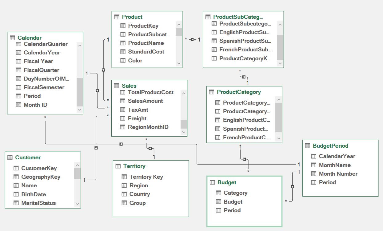
As you can see, the sales data is stored in the Sales table and the Budget data is stored in the Budget table. The Sales table contains each transaction at the product level whereas the Budget data is summarized by Category and Period. Also, the Budget table cannot be joined with the Calendar table as 1:N relationship. As such, we will not be able to combine these two tables in a Pivot Table report for comparison purposes (Budget vs Actual).

Therefore, I used the following steps to create a free form report that contains data from both tables and added columns to calculate the variance and variance %.

1. Created a pivot table from the Sales table.

2. Created a pivot table from the Budget table.

3. Converted both pivot tables to convert Pivot Table to Formulas (OLAP Tools > Convert to Formulas).

4. Created a combined report by copying and pasting formulas from the above two reports.

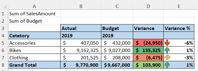
5. Added Variance and Variance % columns.

Here’s the resulting free form report.

Here’s the report showing underlying formulas.

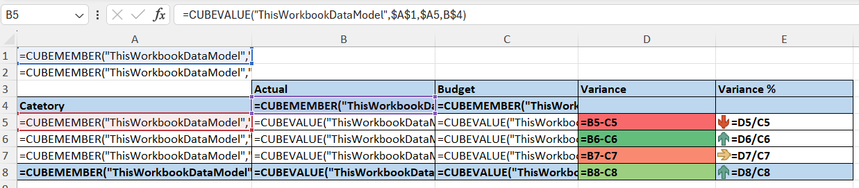
The report uses the following two Cube functions:

CUBEMEMBER

CUBEVALUE

You can get more details on creating free form reports using Cube functions from the original post here.

Excel Fun!

Last Friday’s Morning Brew newsletter contained the following math puzzle.

Friday puzzle

In a small village, 90% of people drink tea, 80% coffee, 70% whiskey, 60% gin. Nobody drinks all four. What percentage of people drink alcohol?

The puzzle looks deceptively simple but it takes some work to solve it.

It is possible to solve the puzzle using logic and math. However, I wanted to find out if I could use Microsoft Excel to solve the puzzle with the help of the Solver add-in.

If you like solving math puzzles, you may want to pause here and attempt to solve the puzzle on your own. Otherwise, read on.

This is how I set up the puzzle in Excel for the Solver to solve.

The table contains the drinks (tea, coffee, whiskey and gin) as rows and ten 10% segments of the population as columns of the table. Each cell ($B$2:$K$5) in the table contains 1 if the population segment takes the drink and 0 if it does not.

We are now ready to set up the Solver Parameters.

We know the following:

1. Percentage of tea drinkers is 90%, coffee 80%, whiskey 70% and gin 60%.

2. Nobody drinks all four drinks i.e. none of the 10% segments in the table drinks more than 3 drinks.

Based on this information we can set up the Solver Parameters as follows:

Objective:

Assuming that there is only one solution, you can select either Min or Max for the Percentage of alcohol drinkers (cell $L$9). You can also try both options to ensure that the solution is unique.

By Changing Variable Cells:

Contents of the table i.e. $B$2:$K$5. Solver will try changing values in these cells to find the solution that meets the constraints below.

Subject to the Constraints:

1. Each cell in the table must be either 0 or 1 i.e. Binary.

2. Sumproduct for each row must be equal to the specified percentage (90%, 80%, etc.).

3. Total of each column must be less than or equal to 3 (because nobody drinks more than 3 drinks).

Solving Method:

Evolutionary

For the explanation of Solving Methods, refer to: Excel Solver: Which Solving Method Should I Choose? - EngineerExcel

Click “Solve” to solve the problem.

You can view the solution in the screenshot above. Green cells indicate drinkers and red cells indicate non-drinkers. Cell $L$9 shows that the percentage of people that drink alcohol is 100% (the answer to the puzzle) i.e. everyone in the village drinks alcohol. 30% drink both whiskey and gin and the remaining 70% drink one of the two.

You can download the Excel workbook here.

Note: You will need to load the Solver add-in to view the Solver Parameters and solve the problem.

I would love to hear about any math or stats puzzles you have solved using Excel!

Workaround for passing TABLE reference to Excel LAMBDA function

You can use the new LAMBDA function in Excel (Desktop edition) to create custom, reusable functions and call them by a friendly name. The custom function is available throughout the workbook and can be called like native Excel functions.

The Excel Labs (formerly Advanced Formula Environment) add-in’s Import from Grid feature can be used to create the LAMBDA function from an example you create.

For the purpose of this article, I wanted to create a LAMBDA function to calculate the financial ratio (Receivables Turnover ratio for this example) from the Trial Balance table exported from Quickbooks Online. However, any Trial Balance table can be used as long as it follows the format used for this table. The following screenshot shows the part of the table used in this example.

The function takes the Financial Year as a parameter and calculates the Receivable Turnover ratio as follows:

Receivable Turnover = Revenue / Average of Beginning and Ending Accounts Receivable

I started by building my example (B2:E2) using the SUMIFS function as shown in the screenshot below.

I then used the Excel Labs add-in’s Import from Grid feature to build the LAMBDA function.

However, the add-in produced the following error because the Table reference cannot be used in the LAMBDA function.

A workaround for this limitation is to use the INDIRECT function to reference the required tables and columns in the LAMBDA formula. I changed the formulas as shown in the screenshot below.

=SUMIFS(

INDIRECT("TrialBalance[Balance]"),

INDIRECT("TrialBalance[Financial Year]"),A2,

INDIRECT("TrialBalance[Account Type]"),"Accounts Receivable (A/R)"

)

Clicking the Preview button generated the following code with a warning:

The warning is related to the INDIRECT function. The INDIRECT function is volatile because the range of the table is unknown and can change. As such it may cause the entire workbook to be recalculated frequently. Volatile functions can impact performance, especially for large workbooks. You can set the "Manual" calculation option to avoid automatic recalculation.

Here is the complete LAMBDA function generated by the add-in:

RecvTO = LAMBDA(FinYear,

    LET(

        EndAR, SUMIFS(

            INDIRECT(

                "TrialBalance[Balance]"

            ),

            INDIRECT(

                "TrialBalance[Financial Year]"

            ), FinYear,

            INDIRECT(

                "TrialBalance[Account Type]"

            ), "Accounts Receivable (A/R)"

        ),

        BegAR, SUMIFS(

            INDIRECT(

                "TrialBalance[Balance]"

            ),

            INDIRECT(

                "TrialBalance[Financial Year]"

            ), FinYear - 1,

            INDIRECT(

                "TrialBalance[Account Type]"

            ), "Accounts Receivable (A/R)"

        ),

        Revenue, SUMIFS(

            INDIRECT(

                "TrialBalance[Balance]"

            ),

            INDIRECT(

                "TrialBalance[Financial Year]"

            ), FinYear,

            INDIRECT(

                "TrialBalance[Account Type]"

            ), "Income"

        ) * -1,

        Revenue /

            ((EndAR + BegAR) / 2)

    )

);

You can verify your custom function by entering it in any cell. See the F2 cell below containing the custom function: =RecvTO(A2).

You can download the above Excel workbook here. Note that you will need to install the Excel Labs add-in to use the Import from Grid feature.

Use Action to retrieve or update data in an unrelated entity in Dynamics 365 Workflows

There are scenarios where you need to access data from an entity that is not directly related to the entity for which you are building a Workflow in Dynamics 365.

For example, you want to send an email alert to the Owner of the Account on the Opportunity when an Opportunity Line is created or updated with the amount exceeding $10,000. In this case, the Workflow will be created for the Opportunity Line entity which triggers the Workflow. However, within the Workflow Designer, you can access data only from the entities that are reated to Opportunity Line entity such as Opportunity or Product. However, Account is not directly related to the Opportunity Line entity and therefore you cannot access the Owner field of the Account within the Workflow. To get around this limitation, you can create another Process of type Action. The Action will be for the Account entity and it will return the Entity Reference for the Account being passed to the Action. You can then call (perform) this Action within your Workflow. This will enable you to access any fields from the Account entity within the Workflow. Here are the specific steps to implement this solution.

Create a Process of type Action on the Account entity.

Add an Argument of Type EntityReference returning the Account entity as Output.

Add the Assign Value step as shown in the screenshot below.

Activate the Action.

Next, create a Workflow for the Opportunity Line entity.

Select "Record is created" and "Record fields change" (Line Amount) triggers.

Add condition. In this case it is: if Opportunity Line:Amount > 10,000.

Add the Perform Action step and select the Action created above.

Pass the Account on the Opportunity as the Input parameter.

Add the Send Email step.

As you can see from the screenshot below, you can now access the Owner field on the Account to populate the “To” (email recipient) in the Send Email step.

Complete the other details for your email.

Activate the Workflow and test your Workflow by adding or updating a line on the Opportunity exceeding $10,000.

You can use this Action in other Workflows or code where you need to retrieve data from a specific Account record.

In addition, you can use this technique to update an unrelated record in your Workflow which was not previously possible.

You can also use this technique to retrieve data from the Business Unit of the record owner
or Field Service Settings which are not directly related to the record on which the Workflow is being executed.

In this post, we saw how you can retrieve or update data in an unrelated entity within the Workflow using Action.